The Fit Wizard

Select Function Tab

The top of the dialog box is used to select one of the four Categories of functions:

To choose a function, first select a category and then the desired function from the displayed Function list.

If the selected function is from the Built-in category and you wish to perform the fit operation using the selected built-in model, you must check the option Fit using built-in function. This will clear the contents of the edit text pane (see image below) and copy the selected function into it.

If the selected built-in model is one of the following peak shape functions: Gauss, Lorentz, PsdVoigt1 or PsdVoigt2, the Peaks input box becomes available, allowing to choose the number of individual peaks for a multi-peak fit operation.

When the selected built-in model is the Polynomial function the Polynomial order input box becomes available, allowing to choose the order of the polynomial fit function.

If you wish to define your own fit model, the Fit using built-in function option should be unchecked. In this case you can also click the Add expression button to copy the selected function, but this will not clear any previous contents from the edit text pane. If you've selected one of the Basic functions, there are no checkboxes/options available and you need to use the Add expression button.

The bottom half of the dialog box allows you to define your own function. You can either write you own mathematical expression from scratch or add expressions from the function selector with the Add expression button. Once a custom expression is completed, clicking on the Save button will add the function to the list of user defined functions. The Name field will be used as the name of the function. A copy of the function is saved on disk with the extension ".fit". You can define the folder where ".fit" files are saved using either the Choose models folder... button (shown only when "User defined" is selected) or by selecting a new folder in the Save file dialog. Functions can be removed from the User Defined list by selecting them and clicking on the Remove button. You will be asked to confirm the deletion.

Fitting Session Tab

In this second step the parameters of the fit must be defined. A starting point must be provided for the fitting parameters usig the Initial guesses tab.

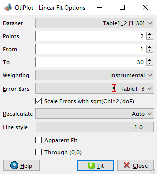
In the Data Set tab you can choose the input data set(s) and also choose a weighting method for your fit (the default is No weighting). The available weighting methods are:

1. No weight: all weighting coefficients are set to 1 (w_i = 1).

2. Instrumental: the values of the associated error bars are used as weighting coefficients w_i = 1/er_i², where er_i are the error bar sizes stored in error bar columns. You must add error bars to the analyzed curve before performing the fit.

3. Statistical: the weighting coefficients are calculated as w_i = 1/y_i, where y_i are the y values in the fitted data set.

4. Arbitrary Dataset: allows setting the weighting coefficients using an arbitrary data set w_i = 1/c_i², where c_i are the values in the arbitrary data set. The column used for the weighting must have a number of rows equal to the number of points in the fitted curve.

5. Direct Weighting: allows setting the weighting coefficients using an arbitrary data set w_i = c_i, where c_i are the values in the arbitrary data set. The column used for the weighting must have a number of rows equal to the number of points in the fitted curve.

It is also possible to specify how the fit operation responds to modifications of the source data curve using the Recalculate list box. The available options are:

The recalculation mode can be changed later on via the Analysis tab of the plot details dialog.

Custom Output Tab

Depending on the settings in the Custom Output tab, a function curve (option Uniform X Function) or a new table (if you choose the option Same X as Fitting Data) will be created for each fit. The new table includes all the X and Y values used to compute and to plot the fitted function and is hidden by default. It can be found in and viewed from the project explorer.

After the fit, if the Write Parameters to Result Log box from the Options group is checked, the log window is opened to show the results of the fitting process.

The options in the Curves group box can be used to specify if some additional plot curves should be generated after each fit operation. If the Conf. Bands and Pred. Bands options are checked QtiPlot generates confidence bands and prediction bands for the current fit, based on the user defined value for the confidence level. If the Residuals Plot option is checked the curve of the fit residuals is also displayed. The residuals are calculated as the difference between the experimental Y_i values and the response values predicted by the fit model.

The controls in the Parameters Output group box can be used in order to define the options for the display of the results from data fit operations. The Format list box allows to choose a default numerical format. The value of the Significant Digits option can be used to customize the precision of the output and has a different meaning depending on the numeric format. The following format and precision options are available: